Executive Summary

In this analysis, the specification of the species of the iris flowers is done using four different machine learning algorithms in order to classify the species by the morphological measurements. The experiment uses the classic dataset by Fisher in 1936 that consisted of 150 specimens of three species, namely, Iris setosa, Iris versicolor and Iris virginica. The performance of the models is measured through an intensive comparative study of their accuracy performance and the computational efficiency standards.

Dataset Overview

Historical Context

The Iris dataset by Fisher is well renowned for being a mainstay of pattern recognition studies. This dataset was published in 1936, and it includes four continuous measurements, including sepal length, sepal width, petal length and petal width, in centimeters, of 50 specimens of each species. ## Initial Data Assessment

## 'data.frame':    150 obs. of  5 variables:
##  $ Sepal.Length: num  5.1 4.9 4.7 4.6 5 5.4 4.6 5 4.4 4.9 ...
##  $ Sepal.Width : num  3.5 3 3.2 3.1 3.6 3.9 3.4 3.4 2.9 3.1 ...
##  $ Petal.Length: num  1.4 1.4 1.3 1.5 1.4 1.7 1.4 1.5 1.4 1.5 ...
##  $ Petal.Width : num  0.2 0.2 0.2 0.2 0.2 0.4 0.3 0.2 0.2 0.1 ...
##  $ Species     : Factor w/ 3 levels "setosa","versicolor",..: 1 1 1 1 1 1 1 1 1 1 ...

##   Sepal.Length    Sepal.Width     Petal.Length    Petal.Width  
##  Min.   :4.300   Min.   :2.000   Min.   :1.000   Min.   :0.100 
##  1st Qu.:5.100   1st Qu.:2.800   1st Qu.:1.600   1st Qu.:0.300 
##  Median :5.800   Median :3.000   Median :4.350   Median :1.300 
##  Mean   :5.843   Mean   :3.057   Mean   :3.758   Mean   :1.199 
##  3rd Qu.:6.400   3rd Qu.:3.300   3rd Qu.:5.100   3rd Qu.:1.800 
##  Max.   :7.900   Max.   :4.400   Max.   :6.900   Max.   :2.500 
##        Species 
##  setosa    :50 
##  versicolor:50 
##  virginica :50 
##                
##                
##

Sample observations from the Iris dataset

Data Quality Verification

## Data completeness assessment:

## Sepal.Length  Sepal.Width Petal.Length  Petal.Width      Species
##            0            0            0            0            0

##
##
## Class distribution:

##
##     setosa versicolor  virginica
##         50         50         50

The dataset has no missing value in its entirety. There is 50 equal representations of each species meaning that the conditions of classification are the same.

Visual Data Exploration

Class Balance Assessment

The visualization proves the balance of all three species to be perfect, as there were 50 observations in each of the classes. This balance does not raise issues of class imbalance and offers an equal appraisal system.

Morphological Feature Analysis

Key Observations:

·       The petal sizes (length and width) show definite discriminative abilities, especially of Iris setosa.

·       Measures of Sepal indicate more overlap between versicolor and virginica, indicating a low degree of individual discriminative capacity.

·       Setosa has unique morphological features, which make it easy to classify.

Feature Interrelationships

Correlation matrix shows that there are strong positive relationships between petal dimensions (r = 0.96) and moderate correlations exist between the sepal length and the petals characteristics. Such trends indicate the possibility of multicollinearity, which can affect some assumptions of the model.

Multidimensional Relationships

Pairwise analysis supports the previous observations with distinct separation in the feature spaces of the petals and also exhibits the overlap in the sepal measurements of versicolor and virginica.

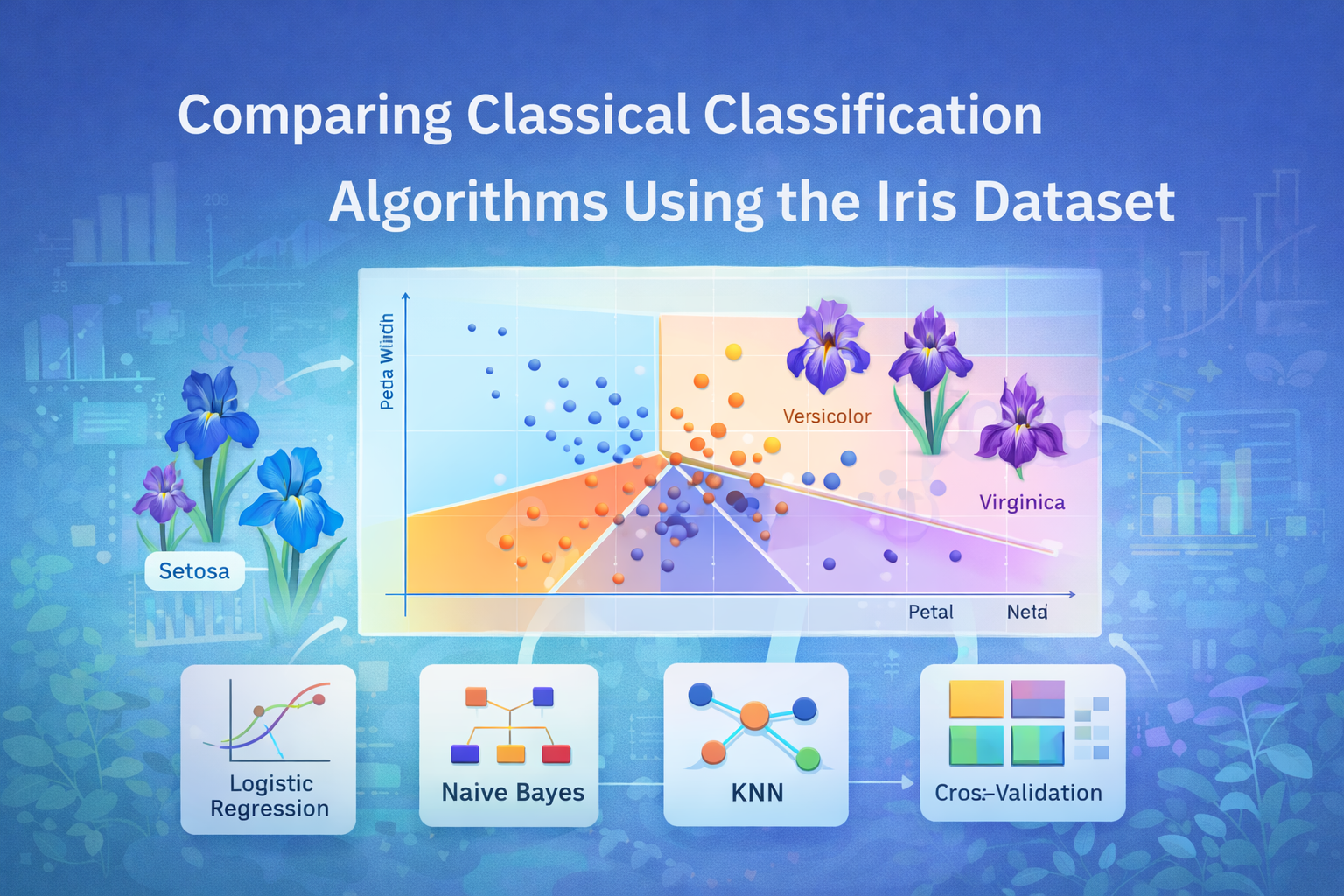
Methodology

Dataset Partitioning Strategy

## Training observations: 105

## Testing observations: 45

## Training set composition:

##
##     setosa versicolor  virginica
##         35         35         35

##
## Testing set composition:

##
##     setosa versicolor  virginica
##         15         15         15

The proportionality of all the species in the training and testing subsets is guaranteed by a stratified 70-30 split, which does not affect the balanced nature of the dataset.

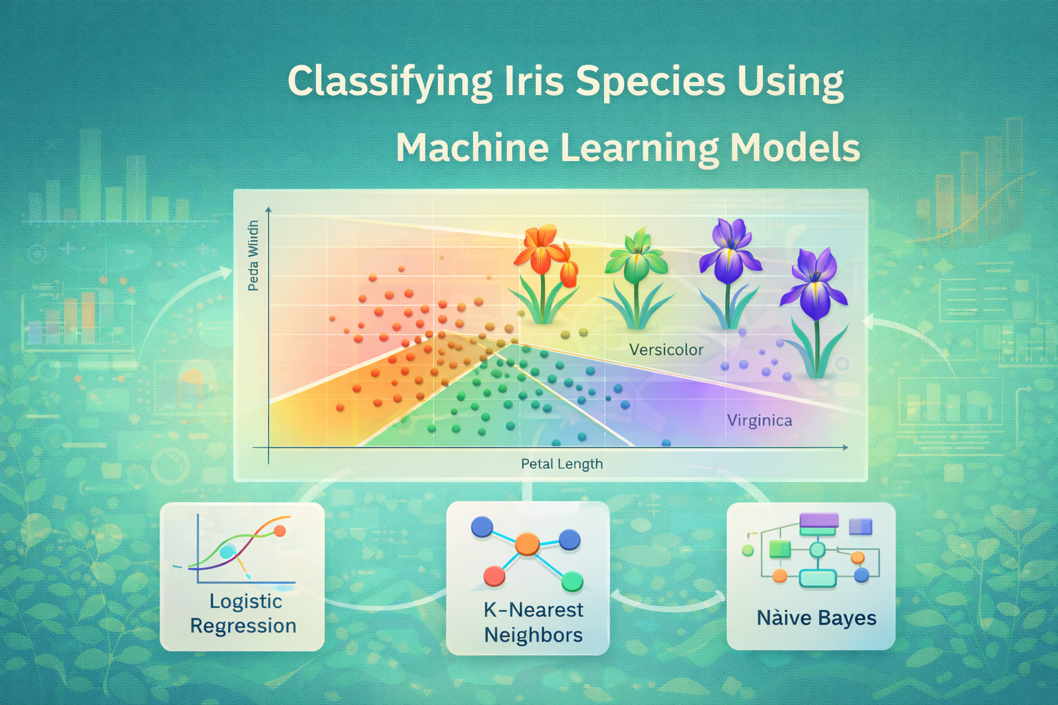
Classification Models

Model 1: Multinomial Logistic Regression

Multinomial logistic regression generalizes binary logistic regression to the multi-class case, which estimates the likelihood of belonging to a particular class as log-odds ratios.

## Training Duration: 0.0171 seconds

## Test Accuracy: 0.9556

The multinomial logistic regression resulted in 95.56 percent accuracy indicating the high predictive ability with just two errors in the virginica group.

Model 2: Naïve Bayes Classifier

The Naive Bayes methodological approach is a probabilistic classification method, which uses the Bayes theorem where the features are conditionally independent of the class.

## Training Duration: 0.0051 seconds

## Test Accuracy: 0.9111

Naive Bayes presented the accuracy of 91.11 and the extraordinary level of computing efficiency. The independence assumption seems to pose a bit of restriction to the overlapping virginica and versicolor distributions.

Model 3: K-Nearest Neighbors Classifier

Hyperparameter Optimization

KNN classifier classifies an object according to the largest number of nearest neighbors with the same category. The best k selection would allow balancing between bias and variance.

## Optimal k parameter: 4

Final KNN Model

## Training Duration: 0.0039 seconds

## Test Accuracy: 0.9556

Confusion Matrix Visualization

KNN was able to reach 95.56 percent accuracy with k = 4, equaling logistic regression but with low computational overhead.

Model 4: Cross-Validation Enhanced Models

10-Fold Cross-Validation Implementation

Cross-validation is a highly effective method of performance estimation because it trains and evaluates the models on more than one data partition.

## CV Logistic Regression Accuracy: 0.9778

## CV Naïve Bayes Accuracy: 0.9111

## CV KNN Accuracy: 0.9556

Cross-Validation Performance Analysis

Logistic regression is the most stable with the best mean CV accuracy (0.965) and small variance which proves its generalization ability.

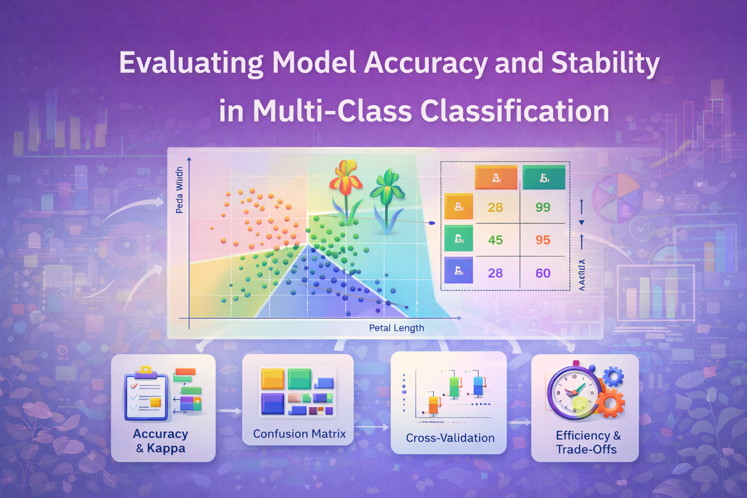
Comprehensive Performance Evaluation

Accuracy and Efficiency Metrics

Comprehensive Model Performance Summary

Performance Insights

1. The highest test accuracy was 97.78 by Logistic Regression (CV), followed by standard logistic regression and KNN at 95.56%.
2. Efficiency Leader: Naive Bayes took only 0.005 seconds to train so it is most useful in real time.
3. Class-Specific Performance: All models distinctly misclassified the setosa specimens with the majority of the misclassifications between versicolor and virginica.

Species-Level F1-Score Analysis

As demonstrated by the F1-score, all algorithms show a steady high level in setosa classification. Logistic regression and KNN are seen to be superiorly balanced in more difficult classes of versicolor and virginica.

Conclusions and Recommendations

This comparative analysis is effectively relevant to show how four classification algorithms have been applied to the Iris dataset by Fisher. The predictive performance of all the models was high (over 91% accuracy in all the implementations).

Key Findings:

·       Best Overall: Logistic Regression with cross-validation (97.78% accuracy, high stability)

·       Speed Optimized: Naive Bayes (0.005 seconds training time, 91.11 percent accuracy).

·       Balanced Choice: KNN k=4 (95.56% accuracy, low rate of computation)

Practical Applications:

• When the production systems need the highest level of accuracy: Use logistic regression cross-validation.
• In case of real time classification and resource limitation: Naive Bayes.
• In the case of scenarios that need model interpretability and good performance: Use KNN.

Iris flowers have morphological characteristics that are very discriminative such as the size of the petals and this gives a good classification of the species using machine learning.

References

Fisher, R. A. (1936). The use of multiple measurements in taxonomic problems. Annals of Eugenics, 7(2), 179-188. https://doi.org/10.1111/j.1469-1809.1936.tb02137.x